If you see this, something is wrong

Collapse and expand sections

To get acquainted with the document, the best thing to do is to select the "Collapse all sections" item from the "View" menu. This will leave visible only the titles of the top-level sections.

Clicking on a section title toggles the visibility of the section content. If you have collapsed all of the sections, this will let you discover the document progressively, from the top-level sections to the lower-level ones.

Cross-references and related material

Generally speaking, anything that is blue is clickable.

Clicking on a reference link (like an equation number, for instance) will display the reference as close as possible, without breaking the layout. Clicking on the displayed content or on the reference link hides the content. This is recursive: if the content includes a reference, clicking on it will have the same effect. These "links" are not necessarily numbers, as it is possible in LaTeX2Web to use full text for a reference.

Clicking on a bibliographical reference (i.e., a number within brackets) will display the reference.

Speech bubbles indicate a footnote. Click on the bubble to reveal the footnote (there is no page in a web document, so footnotes are placed inside the text flow). Acronyms work the same way as footnotes, except that you have the acronym instead of the speech bubble.

Discussions

By default, discussions are open in a document. Click on the discussion button below to reveal the discussion thread. However, you must be registered to participate in the discussion.

If a thread has been initialized, you can reply to it. Any modification to any comment, or a reply to it, in the discussion is signified by email to the owner of the document and to the author of the comment.

First published on Thursday, Jan 9, 2025 and last modified on Thursday, Jan 9, 2025 by Fabienne Chaplais.

I am normally hidden by the status bar

Linear Algebra in the Euclidian Space: Section 8 Test Corrected

Fabienne Chaplais Mathedu

Keywords: Complex Numbers, Polygon

1 Draw an Hexagon and Save the Figure

1.1 Configure Spyder for the figure

Your Spyder doesn’t draw necessarily the figure in an independent window, so that it may be saved on your device.

To do this, go to the ‘preferences’ in the ‘Python’ menu.

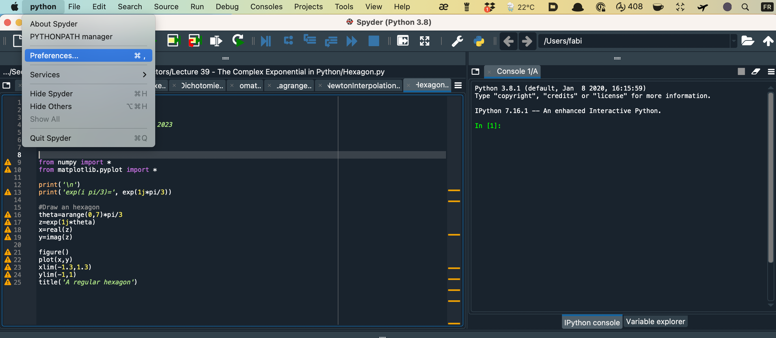
Then you select ‘Python Console’ in the left and then ‘Graphics’ upwoards.

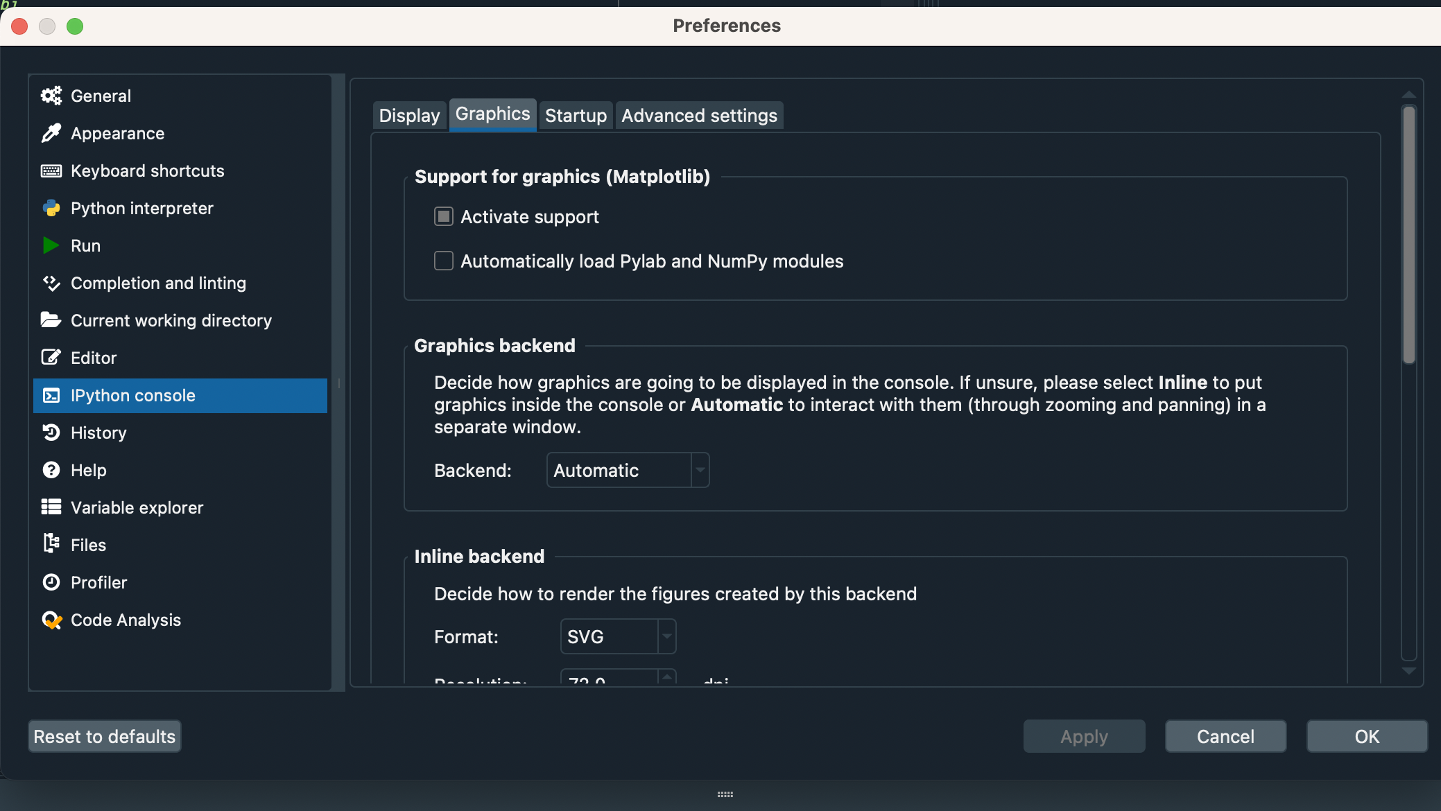
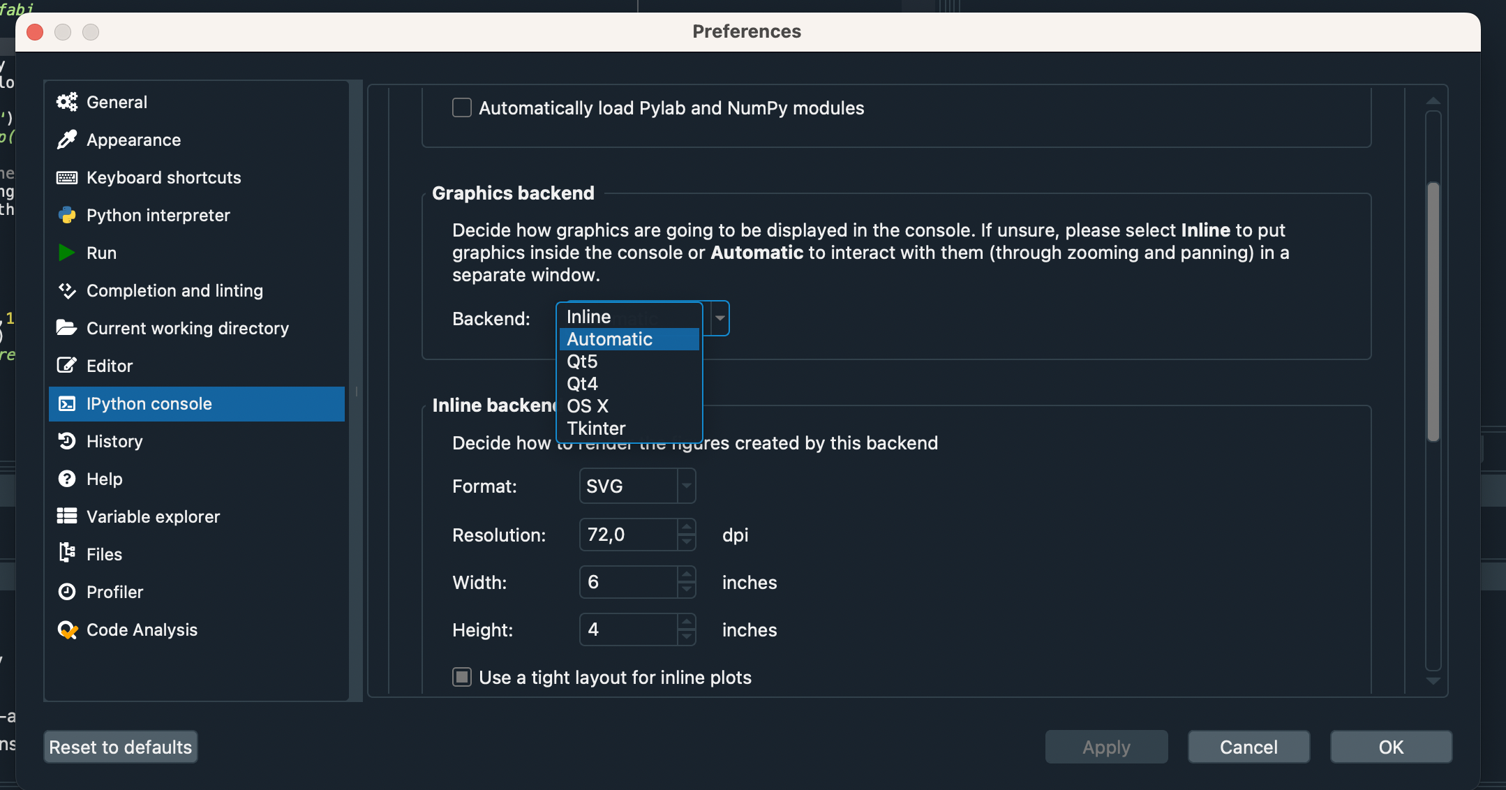
Then you check the pop-up menu ‘Backend’ to ‘Automatic’ and you save.

After all of it, you quit Spyder and relaunch it.

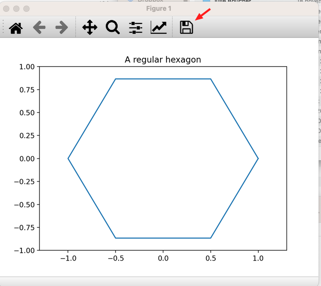
1.2 Script to Draw the Hexagon

Here is the script to draw an hexagon.

from numpy import *
	from matplotlib.pyplot import *
	
	#Draw an hexagon
	theta=arange(0,7)*pi/3
	# real numbers from 0 to 6*pi/3=2*pi, by steps of pi\3=2*pi/6
	z=exp(1j*theta)
	x=real(z)
	y=imag(z)
	
	figure()
	plot(x,y)
	xlim(-1.3,1.3)
	ylim(-1,1)
	title(&apos;A regular hexagon&apos;)

Just copy and paste it in Spyder text editor, save it and run it.

Once you have the figure, save it by clicking on the floppy disk at the upper right corner.

2 Question 1: Draw a Pentagon

Adapt the sript to draw a pentagon, with 5 sides instead of 6.

Please copy and paste in your answer the validated script.

Run it and save the figure you obtain, naming it ‘Pentagon.png’.

Copy and paste it in your answer.

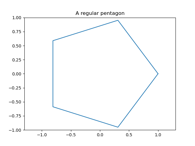
2.1 Solution

The script is the following.

from numpy import *
	from matplotlib.pyplot import *
	
	#Draw a pentagon
	theta=arange(0,6)*2*pi/5
	# real numbers from 0 to 5*2*pi/5=2*pi, by steps of 2*pi/5
	z=exp(1j*theta)
	x=real(z)
	y=imag(z)
	
	figure()
	plot(x,y)
	xlim(-1.3,1.3)
	ylim(-1,1)
	title(&apos;A regular pentagon&apos;)

The figure is the following:

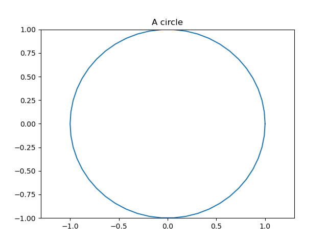
3 Question 2: Draw a Circle

To approximate a circle, dapt the sript to draw a polygon with 50 sides, to draw a pentagon.