If you see this, something is wrong

LaTeX2Web, a web authoring and publishing system
LaTeX2Web, a web authoring and publishing system
Table of contents
Digest for "Lecture Notes on Quantum Algorithms for Scientific Computation"
Example 1 (Single qubit system)
A (single) qubit corresponds to a state space \( \mathcal{H}\cong\mathbb{C}^2\) . We also define
(5)
Since the state space of the spin-\( \frac12\) system is also isomorphic to \( \mathbb{C}^2\) , this is also called the single spin system, where \( \ket{0},\ket{1}\) are referred to as the spin-up and spin-down state, respectively. A general state vector in \( \mathcal{H}\) takes the form
(6)
and the normalization condition implies \( \left\lvert a\right\rvert ^2+\left\lvert b\right\rvert ^2=1\) . So we may rewrite \( \ket{\psi}\) as
(7)
If we ignore the irrelevant global phase \( \gamma\) , the state is effectively
(8)
So we may identify each single qubit quantum state with a unique point on the unit three-dimensional sphere (called the Bloch sphere) as
(9)
Example 2
For a single qubit, the Pauli matrices are
(11)
Together with the two-dimensional identity matrix, they form a basis of all linear operators on \( \mathbb{C}^2\) .
Example 3
Let the Hamiltonian \( H\) be the Pauli-X gate. Then
(18)
Starting from an initial state \( \ket{\psi(0)}=\ket{0}\) , after time \( t=\pi/2\) , the state evolves into \( \ket{\psi(\pi/2)}=-\mathrm{i} \ket{1}\) , i.e., the \( \ket{1}\) state (up to a global phase factor).
Example 4
Again let \( M=X\) . From the spectral decomposition of \( X\) :
(25)
where \( \ket{\pm}:=\frac{1}{\sqrt{2}}(\ket{0}\pm\ket{1}), \lambda_{\pm}=\pm 1\) , we obtain the eigendecomposition
(26)
Consider a quantum state \( \ket{\psi}=\ket{0}=\frac{1}{\sqrt{2}}(\ket{+}+\ket{-})\) , then
(27)
Therefore the expectation value of the measurement is \( \braket{\psi|M|\psi}=0.\)
Example 5 (Two qubit system)
The state space is \( \mathcal{H}=(\mathbb{C}^2)^{\otimes 2}\cong \mathbb{C}^{4}\) . The standard basis is (row-major order, i.e., last index is the fastest changing one)
(31)
The Bell state (also called the EPR pair) is defined to be
(32)
which cannot be written as any product state \( \ket{a}\otimes\ket{b}\) ( 4).
There are many important quantum operators on the two-qubit quantum system. One of them is the CNOT gate, with matrix representation
(33)
In other words, when acting on the standard basis, we have
(34)
This can be compactly written as
(35)
Here \( a\oplus b=(a+b)\mod 2\) is the “exclusive or” (XOR) operation.
Example 6 (Multi-qubit Pauli operators)
For a \( n\) -qubit quantum system, the Pauli operator acting on the \( i\) -th qubit is denoted by \( P_i\) (\( P=X,Y,Z\) ). For instance
(36)
Example 7 (Reduced density operator of tensor product states)
If \( \rho_{AB}=\rho_1\otimes \rho_2\) , then
(43)
Example 8
Let us verify that the CNOT gate does not violate the no-cloning theorem, i.e., it cannot be used to copy a superposition of classical bits \( \ket{x}=a\ket{0}+b\ket{1}\) . Direct calculation shows
(52)
In particular, if \( \ket{x}=\ket{+}\) , then CNOT creates a Bell state.
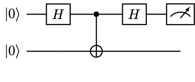
Example 9 (Deferring quantum measurements)
Consider the circuit
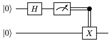
Here the double line denotes the classical control operation. The outcome is that qubit \( 0\) has probability \( 1/2\) of outputting \( 0\) , and the qubit \( 1\) is at state \( \ket{0}\) . Qubit \( 0\) also has probability \( 1/2\) of outputting \( 1\) , and the qubit \( 1\) is at state \( \ket{1}\) .
However, we may replace the classical control operation after the measurement by a quantum controlled \( X\) (which is CNOT), and measure the qubit \( 0\) afterwards:
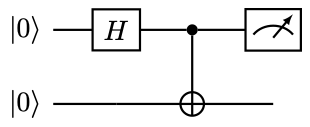
It can be verified that the result is the same. Note that CNOT acts as the classical copying operation. So qubit \( 1\) really stores the classical information (i.e., in the computational basis) of qubit \( 0\) .
Example 10 (Deferred measurement requires extra qubits)
The procedure of deferring quantum measurements using CNOTs is general, and important. Consider the following circuit:
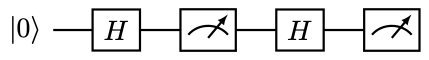
The probability of obtaining \( 0,1\) is \( 1/2\) , respectively. However, if we simply “defer” the measurement to the end by removing the intermediate measurement, we obtain
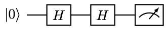
The result of the measurement is deterministically \( 0\) ! The correct way of deferring the intermediate quantum measurement is to introduce another qubit
Measuring the qubit \( 0\) , we obtain \( 0\) or \( 1\) w.p. \( 1/2\) , respectively. Hence when deferring quantum measurements, it is necessary to store the intermediate information in extra (ancilla) qubits, even if such information is not used afterwards.
Example 11 (Estimating success probability on one qubit)
Let \( A\) be the single qubit to be measured in the computational basis, and we are interested in the accuracy in estimating the success probability of obtaining \( 1\) , i.e., \( p\) . This can be realized as an expectation value with \( M_A=\ket{1}\bra{1}\) , and \( p=\operatorname{Tr}\) . Note that \( M_A^2=M_A\) , then
(60)
Hence to estimate \( p\) to additive error \( \epsilon\) , the number of samples needed satisfies
(61)
Note that if \( p\) is close to \( 0\) or \( 1\) , the number of samples needed is also very small: indeed, the outcome of the measurement becomes increasing deterministic in this case!
If we are interested in estimating \( p\) to multiplicative accuracy \( \epsilon\) , then the number of samples is
(62)
and the task becomes increasingly more difficult when \( p\) approaches \( 0\) .
Proposition 1 (Hybrid argument)
Given unitaries \( U_1,\widetilde{U}_1,…, U_K,\widetilde{U}_K\in\mathbb{C}^{N\times N}\) satisfying
(63)
we have
(64)
Proposition 2 (Duhamel’s principle for Hamiltonian simulation)
Let \( U(t),\widetilde{U}(t)\in \mathbb{C}^{N\times N}\) satisfy
(67)
where \( H\in \mathbb{C}^{N\times N}\) is a Hermitian matrix, and \( B(t)\in \mathbb{C}^{N\times N}\) is an arbitrary matrix. Then
(68)
and
(69)
Theorem 1 (Solovay-Kitaev)
Let \( \mathcal{S},\mathcal{T}\) be two universal gate sets that are closed under inverses. Then any \( m\) -gate circuit using the gate set \( \mathcal{S}\) can be implemented to precision \( \epsilon\) using a circuit of \( \mathcal{O}(m\cdot \operatorname{poly}\log(m/\epsilon))\) gates from the gate set \( \mathcal{T}\) , and there is a classical algorithm for finding this circuit in time \( \mathcal{O}(m\cdot \operatorname{poly}\log(m/\epsilon))\) .
Remark 1 (Discarding working registers)
After the uncomputation as shown in 2, the first two registers are unchanged before and after the application of the circuit (though they are changed during the intermediate steps). Therefore 2 effectively implements a unitary
(79)
or equivalently
(80)
In the definition of \( V_f\) , all working registers have been discarded (on paper). This allows us to simplify the notation and focus on the essence of the quantum algorithms under study.
Example 12 (Query access to a boolean function)
Let \( f:\{0,1\}^n\to\{0,1\}\) be a boolean function, which can be queried via the following unitary
(87)
This is called a phase kickback, i.e., the value of \( f(x)\) is returned as a phase factor. The phase kickback is an important tool in many quantum algorithms, e.g. Grover’s algorithm. Note that 1) \( U_f\) can be applied to a superposition of states in the computational basis, and 2) Having query access to \( f(x)\) does not mean that we know everything about \( f(x)\) , e.g. finding the set \( \set{x|f(x)=0}\) can still be a difficult task.
Example 13 (Partially specified quantum oracles)
When designing quantum algorithms, it is common that we are not interested in the behavior of the entire unitary matrix \( U_f\) , but only \( U_f\) applied to certain vectors. For instance, for a \( (n+1)\) -qubit state space, we are only interested in
(88)
This means that we have only defined the first block-column of \( U_f\) as (remember that the row-major order is used)
(89)
Here \( A,B\) are \( N\times N\) matrices, and \( *\) stands for an arbitrary \( N\times N\) matrix so that \( U_f\) is unitary. Of course in order to implement \( U_f\) into quantum gates, we still need to specify the content of \( *\) . However, at the conceptual level, the partially specified unitary (88) simplifies the design process of quantum oracles.
Exercise 1
Prove that any unitary matrix \( U\in \mathbb{C}^{N\times N}\) can be written as \( U=e^{\mathrm{i} H}\) , where \( H\) is an Hermitian matrix.
Exercise 2
Prove 26.
Exercise 3
Write down the matrix representation of the SWAP gate, as well as the \( \sqrt{ \operatorname{SWAP} }\) and \( \sqrt{ \operatorname{iSWAP} }\) gates.
Exercise 4
Prove that the Bell state 32 cannot be written as any product state \( \ket{a}\otimes\ket{b}\) .
Exercise 5
Prove 39 holds for a general mixed state \( \rho\) .
Exercise 6
Prove that an ensemble of admissible density operators is also a density operator.
Exercise 7
Prove the no-deleting theorem in 55.
Exercise 8
Work out the circuit for implementing 76 and 78.
Exercise 9
Prove that if \( f:\{0,1\}^n\to\{0,1\}^n\) is a bijection, and we have access to the inverse mapping \( f^{-1}\) , then the mapping \( U_f:\ket{x}\mapsto \ket{f(x)}\) can be implemented on a quantum computer.
Exercise 10
Prove 56 and 57.
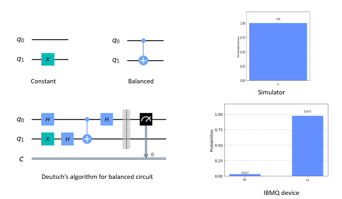
Remark 2 (Deutsch–Jozsa algorithm)
The single-qubit version of the Deutsch algorithm can be naturally generalized to the \( n\) -qubit version, called the Deutsch–Jozsa algorithm. Given \( N=2^n\) boxes with an apple or an orange in each box, and the promise that either 1) all boxes contain the same type of fruit or 2) exactly half of the boxes contain apples and the other half contain oranges, we would like to distinguish the two cases. Mathematically, given the promise that a boolean function \( f:\{0,1\}^n\to\{0,1\}\) is either a constant function (i.e., \( |\set{x|f(x)=0}|=0\) or \( 2^n\) ) or a balanced function (i.e., \( |\set{x|f(x)=0}|=2^{n-1}\) ), we would like to decide to which type \( f\) belongs. We refer to [1, Section 1.4.4] for more details.
Example 14 (Qiskit example of Deutsch’s algorithm)
For \( f(0)=f(1)=1\) (constant case), we can use \( U_f=I\otimes X\) . For \( f(0)=0,f(1)=1\) (balanced case), we can use \( U_f= \operatorname{CNOT} \) .
Remark 3 (Multiple marked states)
The Grover search algorithm can be naturally generalized to the case when there are \( M>1\) marked states. The query complexity is \( \mathcal{O}(\sqrt{N/M})\) .
Example 16 (Reflection with respect to signal qubits)
One common scenario is that the implementation of \( U_{\psi_0}\) requires \( m\) ancilla qubits (also called signal qubits), i.e.,
(119)
where \( \ket{\perp}\) is some orthogonal state satisfying
(120)
Therefore
(121)
This setting is special since the “good” state can be verified by measuring the ancilla qubits after applying \( U_{\psi_0}\) in 119, and post-select the outcome \( 0^m\) . In particular, the expected number of measurements needed to obtain \( \ket{\psi_{\mathrm{good}}}\) is \( 1/p_0\) .
In order to employ the AA procedure, we first note that the reflection operator can be simplified as
(122)
This is because \( \ket{\psi_{\mathrm{good}}}\) can be entirely identified by measuring the ancilla qubits. Meanwhile
(123)
Let \( G=R_{\psi_0}R_{\mathrm{good}}\) , and applying \( G^k\) to \( \ket{\psi_0}\) for some \( k=\mathcal{O}(1/\sqrt{p_0})\) times, we obtain a state that has \( \Omega(1)\) overlap with \( \ket{\psi_{\mathrm{good}}}\) . This achieves the desired quadratic speedup.
Example 17 (Amplitude damping)
Assuming access to an oracle in 119, where \( p_0\) is large, we can easily dampen the amplitude to any number \( \alpha\le \sqrt{p_0}\) .
We introduce an additional signal qubit. Then 119 becomes
(124)
Define a single qubit rotation operation as
(125)
and we have
(126)
Here \( (\ket{0^{m+1}}\bra{0^{m+1}}\otimes I_n)\ket{\perp'}=0\) . We only need to choose \( \sqrt{p_0}\cos \theta=\alpha\) .
Remark 4 (Implication for amplitude amplification)
Due to the close relation between unstructred search and amplitude amplification, it means that given a state \( \ket{\psi}\) of which the amplitude of the “good” component is \( \alpha\ll 1\) , no quantum algorithms can amplify the amplitude to \( \Omega(1)\) using \( o(\alpha^{-\frac12})\) queries to the reflection operators.
Exercise 11
In Deutsch’s algorithm, demonstrate why not assuming access to an oracle \( V_f:\ket{x}\mapsto\ket{f(x)}\) .
Exercise 12
For all possible mappings \( f:\{0,1\}\to\{0,1\}\) , draw the corresponding quantum circuit to implement \( U_f:\ket{x,0}\mapsto\ket{x,f(x)}\) .
Exercise 13
Prove 109.
Exercise 14
Draw the quantum circuit for 117.
Exercise 15
Prove that when ancilla qubits are used, the complexity of the unstructured search problem is still \( \Omega(\sqrt{N})\) .
Example 18 (Overlap estimate using swap test)
An application of the Hadamard test is called the swap test, which is used to estimate the overlap of two quantum states \( \left\lvert \braket{\varphi|\psi}\right\rvert \) . The quantum circuit for the swap test is
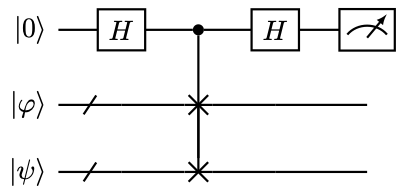
Note that this is exactly the Hadamard test with \( U\) being the \( n\) -qubit swap gate. Direct calculation shows that the probability of measuring the qubit \( 0\) to be in state \( \ket{0}\) is
(150)
Example 19 (Overlap estimate with relative phase information)
In the swap test, the quantum states \( \ket{\varphi},\ket{\psi}\) can be black-box states, and in such a scenario obtaining an estimate to \( \left\lvert \braket{\varphi|\psi}\right\rvert \) is the best one can do. In order to retrieve the relative phase information and to obtain \( \braket{\varphi|\psi}\) , we need to have access to the unitary circuit preparing \( \ket{\varphi},\ket{\psi}\) , i.e.,
(151)
Then we have \( \braket{\varphi|\psi}=\braket{0^n|U_{\varphi}^{†}U_{\psi}|0^n}\) .
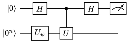
Example 20 (Single qubit phase estimation)
The Hadamard test can also be used to derive the simplest version of the phase estimate based on success probabilities. Apply the Hadamard test in 6 with \( U,\psi\) satisfying 144. Then the probability of measuring the qubit \( 0\) to be in state \( \ket{1}\) is
(152)
Therefore
(153)
In order to quantify the efficiency of the procedure, recall from 11 that if \( p(1)\) is far away from \( 0\) or \( 1\) , i.e., \( (2\varphi \mod 1)\) is far away from \( 0\) , in order to approximate \( p(1)\) (and hence \( \varphi\) ) to additive precision \( \epsilon\) , the number of samples needed is \( \mathcal{O}(1/\epsilon^2)\) .
Now assume \( \varphi\) is very close to \( 0\) and we would like to estimate \( \varphi\) to additive precision \( \epsilon\) . Note that
(154)
Then \( p(1)\) needs to be estimated to precision \( \mathcal{O}(\epsilon^2)\) , and again the number of samples needed is \( \mathcal{O}(1/\epsilon^2)\) . The case when \( \varphi\) is close to \( 1/2\) or \( 1\) is similar.
Note that the circuit in 6 cannot distinguish the sign of \( \varphi\) (or whether \( \varphi\ge 1/2\) when restricted to the interval \( [0,1)\) ). To this end we need 7, but replace \( \mathrm{S}^{†}\) by \( \mathrm{S}\) , so that the success probability of measuring \( 1\) in the computational basis is
(155)
This gives
(156)
Unlike the previous estimate, in order to correctly estimate the sign, we only require \( \mathcal{O}(1)\) accuracy, and run 7 for a constant number of times (unless \( \varphi\) is very close to \( 0\) or \( \pi\) ).
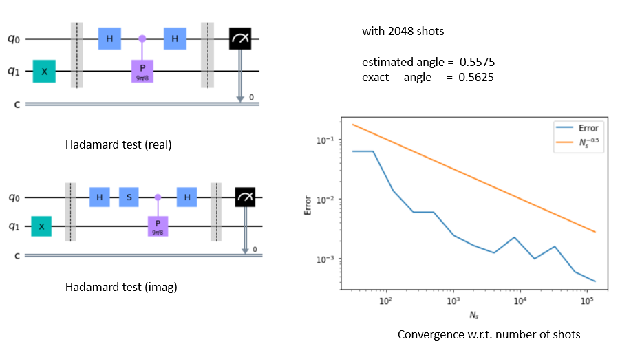
Example 21 (Qiskit example for phase estimation using the Hadamard test)
Here is a qiskit example of the simple phase estimation for
with \( \varphi=0.5+\frac{1}{2^d}\equiv 0.{10… 01}\) (d bits in total). In this example, \( d=4\) and the exact value is \( \varphi=0.5625\) .
Example 22
Consider \( \varphi=0.\varphi_4\varphi_3\varphi_2\varphi_1\varphi_0=0.11111\) and \( d=5\) . Running Kitaev’s algorithm with \( j=0,1,2\) gives the following possible choices of \( \beta_j\) :
Start with \( j=2\) . We have only one choice of \( \beta_j\) , and can recover \( 0.\varphi_2\varphi_1\varphi_0=0.111\) . Then for \( j=1\) , we need to use 161 to decide \( \varphi_3\) . If we choose \( \beta_j=0.111\) , we have \( \varphi_3=1\) . But if we choose \( \beta_j=0.000\) , we still need to choose \( \varphi_3=1\) , since \( \left\lvert .011-0.000\right\rvert _{\bmod 1}=0.100=1/2>1/4\) , and \( \left\lvert .111-0.000\right\rvert _{\bmod 1}=0.001=1/8<1/4\) . Similar analysis shows that for \( j=0\) we have \( \varphi_4=1\) . This recovers \( \varphi\) exactly.
Example 23 (A variant of Kitaev’s algorithm that does not work)
Let us modify Kitaev’s algorithm as follows: for each \( 2^j \varphi\) is determined to precision \( 1/8\) , and round the result to \( \beta_j\in\set{0.00,0.01,0.10,0.11}\) . Start from \( j=d-2\) , we estimate \( .\varphi_1\varphi_0\) exactly. Then for \( j=d-3,…,0\) , we assign
(163)
Now that the inequality \( <1/2\) above can be equivalently written as \( \le 1/4\) .
Let us run the algorithm above for \( \varphi=0.\varphi_4\varphi_3\varphi_2\varphi_1\varphi_0=0.1111\) and \( d=4\) . This gives:
Start with \( j=2\) . We have only one choice of \( \beta_j\) , and can recover \( 0.\varphi_1\varphi_0=0.11\) . Then for \( j=1\) , if we choose \( \beta_j=0.11\) , we have \( \varphi_2=1\) . But if we choose \( \beta_j=0.00\) , then \( \left\lvert .01-0.00\right\rvert _{\bmod 1}=0.0.01=1/4\) , and \( \left\lvert .11-0.000\right\rvert _{\bmod 1}=0.01=1/4\) . So the algorithm cannot distinguish the two possibilities and fails.
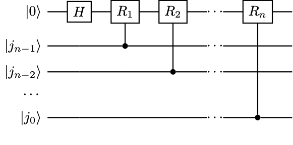
Example 24 (Implementation of controlled rotation)
Consider the implementation of
(176)
Let
(177)
and \( R_j=R_z(\pi/2^{j-1})\) . In particular, \( R_1=Z\) . The quantum circuit is
Example 25 (Qiskit example for QFT)
Remark 5
At first glance, the saving due to the usage of the circuit in 11 may not seem to be large, since we still need to implement matrix powers as high as \( U^{2^{d-1}}\) . However, the alternative would be to implement \( \sum_{j\in[2^d]} \ket{j}\bra{j}\) , which requires very complicated multi-qubit control operations. Another scenario when significant advantage can be gained is when \( U\) can be fast-forwarded, i.e., \( U^j\) can be implemented at a cost that is independent of \( j\) . This is for instance, if \( U=R_z(\theta)\) is a single-qubit rotation. Then the circuit 11 is exponentially better than the direct implementation of \( \mathcal{U}\) .
Example 26 (Hadamard test viewed as QPE)
When \( d=1\) , note that \( U^{†}=U^{†}_{\mathrm{FT}}=H\) , the QFT based QPE in 12 is exactly the Hadamard test in 6. Note that \( \varphi\) does not need to be exactly represented by a one bit number!
Example 27 (Qiskit example for QPE)
Remark 6 (Quantum median method)
One problem with QPE is that in order to obtain a success probability \( 1-\delta\) , we must use \( \log_2 \delta^{-1}\) ancilla qubits, and the maximal simulation time also needs to be increased by a factor \( \delta^{-1}\) . The increase of the maximal simulation time is particularly undesirable since it increases the circuit depth and hence the required coherence time of the quantum device. When \( \ket{\psi}\) is an exact eigenstate, this can be improved by the median method, which uses \( \log \delta^{-1}\) copies of the result from QPE without using ancilla qubits or increasing the circuit depth. When \( \ket{\psi}\) is a linear combination of eigenstates, the problem of the aliasing effect becomes more difficult to handle. One possibility is to generalize the median method into the quantum median method [2], which uses classical arithmetics to evaluate the median using a quantum circuit. To reach success probability \( 1-\delta\) , we still need \( \log_2 \delta^{-1}\) ancilla qubits, but the maximal simulation time does not need to be increased.
Exercise 16
Write down the quantum circuit for the overlap estimate in 19.
Exercise 17
For \( \varphi=0.111111\) , we run Kitaev’s algorithm to estimate its first \( 4\) bits. Check that the outcome satisfies 162. Note that \( 0.0000\) and \( 0.1111\) are both acceptable answers. Prove the validity of Kitaev’s algorithm in general in the sense of 162.
Exercise 18
For a \( 3\) qubit system, explicitly construct the circuit for \( U_{\mathrm{FT}}\) and its inverse.
Exercise 19
For a \( n\) -qubit system, write down the quantum circuit for the swap operation used in QFT.
Exercise 20
Similar to the Hadamard test in 26, develop an algorithm to perform QPE using the circuit in 12 with only \( d=2\) , while the phase \( \varphi\) can be any number in \( [0,1/2)\) .
Example 28 (Transverse field Ising model)
The Hamiltonian for the one dimensional transverse field Ising model (TFIM) with nearest neighbor interaction of length \( n\) is
(195)
The dimension of the Hamiltonian matrix \( H\) is \( 2^n\) .
Example 29 (Fermionic system in second quantization)
For a fermionic system (such as electrons), the Hamiltonian can be expressed in terms of the creation and annihilation operators as
(196)
The creation and annihilation operators \( \hat{a}^{†}_i,\hat{a}_i\) can be converted into Pauli operators via e.g. the Jordan-Wigner transform as
(197)
Here \( X,Y,Z,I\) are single-qubit Pauli-matrices. The dimension of the Hamiltonian matrix \( \hat{H}\) is thus \( 2^n\) .
The number operator takes the form
(198)
For a given state \( \ket{\Psi}\) , the total number of particles is
(199)
The Hamiltonian \( H\) preserves the total number of particles \( N_e\) .
Remark 7 (Dependence on the initial overlap \( p_0\))
The analysis above shows that QPE has a nontrivial dependence on the initial overlap \( p_0\) , which has a rather indirect source. First, in order to reduce the possibility of overshooting, the number of repetitions \( M\) needs to be large enough and is \( \mathcal{O}(p_0^{-1})\) . However, this also increases the probability of undershooting the eigenvalue, and hence \( \delta'\) needs to be chosen to be \( \mathcal{O}(M^{-1})=\mathcal{O}(p_0)\) . This means that the circuit depth should be \( \mathcal{O}(\delta')=\mathcal{O}(p_0^{-1})\) . The total complexity is thus \( TM=\mathcal{O}(p_0^{-2})\) . Therefore, when the initial overlap \( p_0\) is small, using QPE to find the ground state energy can be very costly. On the other hand, using different techniques, the dependence on \( p_0\) can be drastically improved to \( \mathcal{O}(p_0^{-\frac12})\) [3]. See also the discussions in 8.8.
Remark 8 (QPE for preparing the ground state)
The estimate of the ground state energy does not necessarily require the energy gap \( \lambda_g:=\lambda_1-\lambda_0\) to be positive. However, if our goal is to prepare the ground state \( \ket{\psi_0}\) from an initial state \( \ket{\phi}\) using QPE, then we need stronger assumptions. In particular, we cannot afford to obtain \( \ket{k'}\ket{\psi_k}\) , where \( \left\lvert \widetilde{\varphi}_{k'}-\lambda_0\right\rvert <\epsilon\) but \( k\ne 0\) . This at least requires \( \epsilon=2^{-d}<\lambda_g\) , and introduces a natural dependence on the inverse of the gap.
Example 30 (Amplitude estimation to accelerate Hadamard test)
Consider the circuit for the Hadamard test in 6 to estimate \( \operatorname{Re}\braket{\psi|U|\psi}\) . Let the initial state \( \ket{\psi}\) be prepared by a unitary \( U_{\psi}\) , then the following combined circuit
maps \( \ket{0}\ket{0^n}\) to
(223)
and the goal is to estimate \( p_0\) . This also gives the implementation of the reflector \( R_{\psi_0}\) .
Note that \( R_{\mathrm{good}}\) can be implemented by simply reflecting against the signal qubit, i.e.,
(224)
Then we can run QPE to the Grover unitary \( G=R_{\psi_0}R_{\mathrm{good}}\) to estimate \( p(0)\) , and the circuit depth is \( \mathcal{O}(\epsilon^{-1})\) .
Remark 9 (Recovering the norm of the solution)
The HHL algorithm returns the solution to QLSP in the form of a normalized state \( \ket{x}\) stored in the quantum computer. In order to recover the magnitude of the unnormalized solution \( \left\lVert \widetilde{x}\right\rVert \) , we note that the success probability of measuring the signal qubit in 235 is
(238)
Therefore sufficient repetitions of running the circuit in 235 and estimate \( p(1)\) , we can obtain an estimate of \( \left\lVert \widetilde{x}\right\rVert \) .
Proposition 3 (Controlled rotation given rotation angles)
Let \(0\le\theta<1\) has exact \( d\) -bit fixed point representation \(\theta=.\theta_{d-1}…\theta_0\) be its \(d\)-bit fixed point representation. Then there is a \( (d+1)\) -qubit unitary \(U_{\theta}\) such that
(239)
Remark 10 (HHL with amplitude amplification)
We may view 235 as
(254)
Since \( \ket{\psi_{\mathrm{good}}}\) is marked by a single signal qubit, we may use 16 to construct a reflection operator with respect to the signal qubit. This is simply given by
(255)
The reflection with respect to the initial vector is
(256)
where \( U_{\psi_0}=U_{\mathrm{HHL}}(I_1\otimes U_b)\) . Let \( G=R_{\psi_0}R_{\mathrm{good}}\) be the Grover iterate. Then amplitude amplification allows us to apply \( G\) for \( \Theta(p(1)^{-\frac12})\) times to boost the success probability of obtaining \( \ket{\psi_{\mathrm{good}}}\) with constant success probability. Therefore in the worst case when \( p(1)=\Theta(\kappa^{-2})\) , the number of repetitions is reduced to \( \mathcal{O}(\kappa)\) , and the total runtime is \( \mathcal{O}(\kappa^2/\epsilon)\) . This query complexity is the commonly referred query complexity for the HHL algorithm. Note that as usual, amplitude amplification increases the circuit depth. However, the tradeoff is that the circuit depth increases from \( \mathcal{O}(\kappa/\epsilon)\) to \( \mathcal{O}(\kappa^2/\epsilon)\) .
Remark 11 (Comparison with classical iterative linear system solvers)
Let us now compare the cost of the HHL algorithm to that of classical iterative algorithms. If \( A\) is \( n\) -qubit Hermitian positive definite with condition number \( \kappa\) , and is \( d\) -sparse (i.e., each row/column of \( A\) has at most \( d\) nonzero entries), then each matrix vector multiplication \( Ax\) costs \( \mathcal{O}(dN)\) floating point operations. The number of iterations for the steepest descent (SD) algorithm is \( \mathcal{O}(\kappa\log \epsilon^{-1})\) , and the this number can be significantly reduced to \( \mathcal{O}(\sqrt{\kappa}\log \epsilon^{-1})\) by the renowned conjugate gradient (CG) method. Therefore the total cost (or wall clock time) of SD and CG is \( \mathcal{O}(dN\kappa\log \epsilon^{-1})\) and \( \mathcal{O}(dN\sqrt{\kappa}\log \epsilon^{-1})\) , respectively.
On the other hand, the query complexity of the HHL algorithm, even after using the AA algorithm, is still \( \mathcal{O}(\kappa^2/\epsilon)\) . Such a performance is terrible in terms of both \( \kappa\) and \( \epsilon\) . Hence the power of the HHL algorithm, and other QLSP solvers is based on that each application of \( A\) (in this case, using the unitary \( U\) ) is much faster. In particular, if \( U\) can be implemented with \( \operatorname{poly}(n)\) gate complexity (also can be measured by the wall clock time), then the total gate complexity of the HHL algorithm (with AA) is \( \mathcal{O}(\operatorname{poly}(n)\kappa^2/\epsilon)\) . When \( n\) is large enough, we expect that \( \operatorname{poly}(n)\ll N=2^n\) and the HHL algorithm would eventually yield an advantage. Nonetheless, for a realistic problem, the assumption that \( U\) can be implemented with \( \operatorname{poly}(n)\) cost, and no classical algorithm can implement \( Ax\) with \( \operatorname{poly}(n)\) cost should be taken with a grain of salt and carefully examined.
Remark 12 (Readout problem of QLSP)
By solving the QLSP, the solution is stored as a quantum state in the quantum computer. Sometimes the QLSP is only a subproblem of a larger application, so it is sufficient to treat the HHL algorithm (or other QLSP solvers) as a “quantum subroutine”, and leave \( \ket{x}\) in the quantum computer. However, in many applications (such as the solution of Poisson’s equation in 5.4, the goal is to solve the lienar system. Then the information in \( \ket{x}\) must be converted to a measurable classical output.
The most common case is to compute the expectation of some observable \( \braket{O}=\braket{x|O|x}\approx \braket{\widetilde{x}|O|\widetilde{x}}\) . Assuming \( \braket{O}=\Theta(1)\) . Then to reach additive precision \( \epsilon\) of the observable, the number of samples needed is \( \mathcal{O}(\epsilon^{-2})\) . On the other hand, in order to reach precision \( \epsilon\) , the solution vector \( \ket{\widetilde{x}}\) must be solved to precision \( \epsilon\) . Assuming the worst case analysis for the HHL algorithm, the total query complexity needed is
(257)
Remark 13 (Query complexity lower bound)
The cost of a quantum algorithm for solving a generic QLSP scales at least as \( \Omega(\kappa(A))\) , where \( \kappa(A):=\left\lVert A\right\rVert \left\lVert A^{-1}\right\rVert \) is the condition number of \( A\) . The proof is based on converting the QLSP into a Hamiltonian simulation problem, and the lower bound with respect to \( \kappa\) is proved via the “no-fast-forwarding” theorem for simulating generic Hamiltonians [4]. Nonetheless, for specific classes of Hamiltonians, it may still be possible to develop fast algorithms to overcome this lower bound.
Proposition 4 (Diagonalization of tridiagonal matrices)
A Hermitian Toeplitz tridiagonal matrix
(260)
can be analytically diagonalized as
(261)
where \( (v_k)_j=v_{j,k}, j=1,…,N\) , \( b=\left\lvert b\right\rvert e^{\mathrm{i} \theta}\) , and
(262)
Proposition 5
For any \( A\in \mathbb{C}^{N\times N}\) , \( \left\lVert A\right\rVert ^2,(1/\left\lVert A^{-1}\right\rVert )^2\) are given by the largest and smallest eigenvalue of \( A^{†}A\) , respectively.
Theorem 2 (Gershgorin circle theorem, see e.g. {[5, Theorem 7.2.1]})
Let \( A\in\mathbb{C}^{N\times N}\) with entries \( a_{ij}\) . For each \( i=1,…,N\) , define
(277)
Let \( D(a_{ii},R_i)\subseteq \mathbb{C}\) be a closed disc centered at \( a_{ii}\) with radius \( R_i\) , which is called a Gershgorin disc. Then every eigenvalue of \( A\) lies within at least one of the Gershgorin discs \( D(a_{ii},R_i)\)
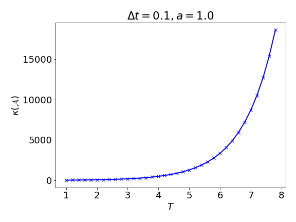
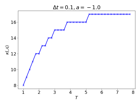
Example 31 (Growth of the condition number when \( \operatorname{Re} a\ge0\))
The Gershgorin circle theorem does not provide a meaningful bound of the condition number when \( \operatorname{Re} a>0\) and \( 1<\left\lvert \xi\right\rvert <2\) . This is a correct behavior. To see this, just consider \( a=1,b=0\) , and the solution should grow exponentially as \( x(T)=e^{T}\) . If \( \kappa(\mathcal{A})=\mathcal{O}\left((\Delta t) ^{-1}\right)\) holds and in particular is independent of the final \( T\) , then the norm of the solution can only grow polynomially in \( T\) , which is a contradiction. See 16 for an illustration. Note that when \( a=-1.0\) , \( \Delta t=0.1\) , the condition number is less than \( 20\) , which is smaller than the upper bound above, i.e., \( 3\times\frac{2}{\Delta t (-a)}=60\) .
Remark 14
It may be tempting to modify the \( (N,N)\) -th entry of \( \mathcal{A}\) to be \( 1+\left\lvert \xi\right\rvert ^2\) to obtain
(288)
Here \( \mathcal{G}\) is a Toeplitz tridiagonal matrix satisfying the requirement of 4. The eigenvalues of \( \mathcal{G}\) take the form
(289)
If we take the approximation \( \lambda_{\min}(\mathcal{A}^{†}\mathcal{A})\approx \lambda_{\min}(\mathcal{G})\) , we would find that 287 holds even when \( \operatorname{Re} a>0\) . This behavior is however incorrect, despite that the matrices \( \mathcal{A}^{†}\mathcal{A}\) and \( \mathcal{G}\) only differ by a single entry!
Proposition 6
For any diagonalizable \( A\in\mathbb{C}^{N\times N}\) with eigenvalue decomposition \( Av_k=\lambda_k v_k\) , we have
(291)
Exercise 21 (Quantum counting)
Given query access to a function \( f:\{0,1\}^N \rightarrow \{0,1\}\) design a quantum algorithm that computes the size of its kernel, i.e.,, total number of \( x\) ’s that satisfy \( f(x)=1\) .
Exercise 22
Consider the initial value problem of the linear differential equation 267.
Construct the linear system of equations
\[ \mathbf{\mathcal{A}} \mathbf{x} = \mathbf{b} \]like 271 using the backward Euler method.
- In the scalar case when \( A(t) \equiv a \in \mathbb{C}\) is a constant satisfying \( \operatorname{Re}(a) \leq 0\) , estimate the query complexity of the HHL algorithm applying to the linear system constructed in (1).
Example 32 (Simulating transverse field Ising model)
For the one dimensional transverse field Ising model (TFIM) with nearest neighbor interaction in 195, wince all Pauli-\( Z_i\) operators commute, we have
(319)
Each \( e^{\mathrm{i} t Z_i Z_{i+1}}\) is a rotation involving only the qubits \( i,j\) , and the splitting has no error. Similarly
(320)
and each \( e^{\mathrm{i} t g X_i}\) can be implemented independently without error.
Example 33 (Particle in a potential)
Let \( H=-\Delta_ř+V(\mathbf{r})=H_1+H_2\) be the Hamiltonian of a particle in a potential field \( V(\mathbf{r})\) , where \( \mathbf{r}\in \Omega=[0,1]^d\) with periodic boundary conditions. After discretization using Fourier modes, \( e^{\mathrm{i} H_1t}\) can be efficiently performed by diagonalizing \( H_1\) in the Fourier space, and \( e^{\mathrm{i} H_2t}\) can be efficiently performed since \( V(\mathbf{r})\) is diagonal in the real space.
Remark 15 (Vector norm bound)
The Hamiltonian simulation problem of interest in practice often concerns the solution with particular types of initial conditions, instead of arbitrary initial conditions. Therefore the operator norm bound in 327 can still be too loose. Taking the initial condition into account, we readily obtain
(330)
For the example of the particle in a potential, we have
(331)
Therefore if we are given the a priori knowledge that \( \max_{0\le s\le t}\left\lVert \psi'(s)\right\rVert =\mathcal{O}(1)\) , we may even have \( L=\mathcal{O}(\epsilon^{-1})\) , i.e., the number of time steps is independent of \( N\) .
Exercise 23
Consider the Hamiltonian simulation problem for \( H = H_1 + H_2 + H_3\) . Show that the first order Trotter formula
has a commutator type error bound.
Exercise 24
Consider the time-dependent Hamiltonian simulation problem for the following controlled Hamiltonian
where \( a(t)\) and \( b(t)\) are smooth functions bounded together with all derivatives. We focus on the following Trotter type splitting, defined as
where the intervals \( [t_j, t_{j+1}]\) are equidistant and of length \( \Delta t\) on the interval \( [0, t]\) with \( t_n = t\) . Show that this method has first-order accuracy, but does not exhibit a commutator type error bound in general.
Definition 1 (Block encoding)
Given an \( n\) -qubit matrix \( A\) , if we can find \( \alpha, \epsilon \in \mathbb{R}_+\) , and an \( (m+n)\) -qubit unitary matrix \( U_A\) so that
(345)
then \( U_A\) is called an \( (\alpha, m, \epsilon)\) -block-encoding of \( A\) . When the block encoding is exact with \( \epsilon=0\) , \( U_A\) is called an \( (\alpha, m)\) -block-encoding of \( A\) . The set of all \( (\alpha, m, \epsilon)\) -block-encoding of \( A\) is denoted by \( \operatorname{BE}_{\alpha,m}(A,\epsilon)\) , and we define \( \operatorname{BE}_{\alpha,m}(A)=\operatorname{BE}(A,0)\) .
Example 34 (\( (1,1)\) -block-encoding is general)
For any \( n\) -qubit matrix \( A\) with \( \left\lVert A\right\rVert _2\le 1\) , the singular value decomposition (SVD) of \( A\) is denoted by \( W\Sigma V^{†}\) , where all singular values in the diagonal matrix \( \Sigma\) belong to \( [0,1]\) . Then we may construct an \( (n+1)\) -qubit unitary matrix
(348)
which is a \( (1,1)\) -block-encoding of \( A\) .
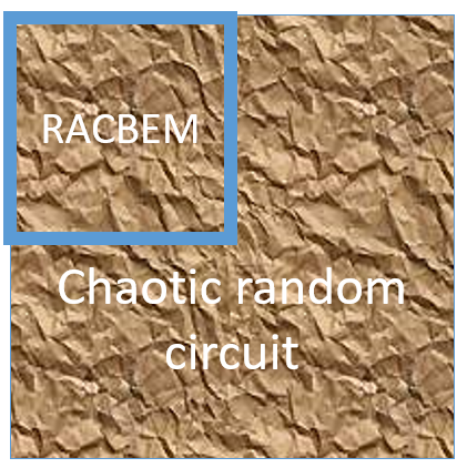
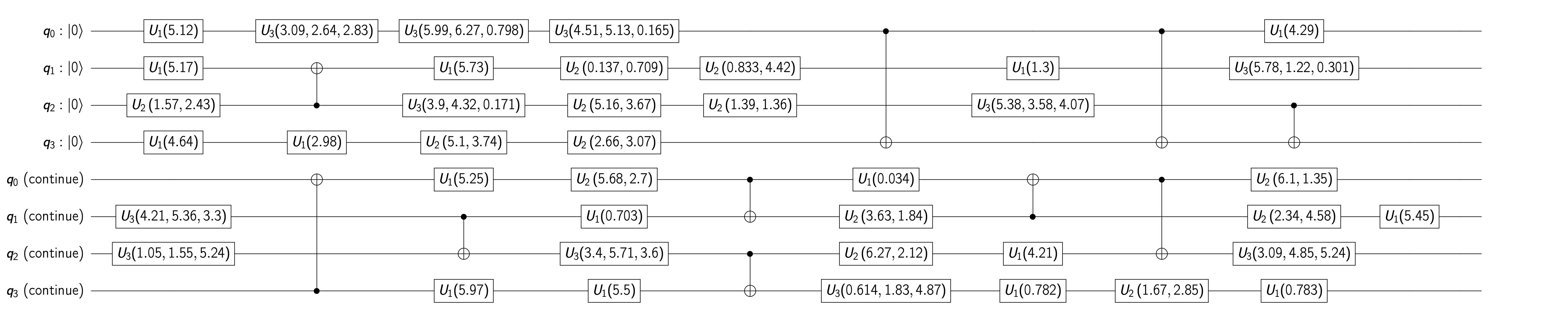
Example 35 (Random circuit block encoded matrix)
In some scenarios, we may want to construct a pseudo-random non-unitary matrix on quantum computers. Note that it would be highly inefficient if we first generate a dense pseudo-random matrix \( A\) classically and then feed it into the quantum computer using e.g. quantum random-access memory (QRAM). Instead we would like to work with matrices that are inherently easy to generate on quantum computers. This inspires the random circuit based block encoding matrix (RACBEM) model [6]. Instead of first identifying \( A\) and then finding its block encoding \( U_A\) , we reverse this thought process: we first identify a unitary \( U_A\) that is easy to implement on a quantum computer, and then ask which matrix can be block encoded by \( U_A\) .
34 shows that in principle, any matrix \( A\) with \( \left\lVert A\right\rVert _2\le 1\) can be accessed via a \( (1,1,0)\) -block-encoding. In other words, \( A\) can be block encoded by an \( (n+1)\) -qubit random unitary \( U_A\) , and \( U_A\) can be constructed using only basic one-qubit unitaries and CNOT gates. The layout of the two-qubit operations can be designed to be compatible with the coupling map of the hardware. A cartoon is shown in 19, and an example is given in 20.
Example 36 (Block encoding of a diagonal matrix)
As a special case, let us consider the block encoding of a diagonal matrix. Since the row and column indices are the same, we may simplify the oracle 333 into
(349)
In the case when the oracle \( \widetilde{O}_A\) is used, we may assume accordingly
(350)
Let \( U_A=O_A\) . Direct calculation shows that for any \( i,j\in [N]\) ,
(351)
This proves that \( U_A\in\operatorname{BE}_{1,1}(A)\) , i.e., \( U_A\) is a \( (1,1)\) -block-encoding of the diagonal matrix \( A\) .
Proposition 7
The circuit in 21 defines \( U_A\in \operatorname{BE}_{s,\mathfrak{s}+1}(A)\) .
Definition 2 (Hermitian block encoding)
Let \( U_A\) be an \( (\alpha, m, \epsilon)\) -block-encoding of \( A\) . If \( U_A\) is also Hermitian, then it is called an \( (\alpha, m, \epsilon)\) -Hermitian-block-encoding of \( A\) . When \( \epsilon=0\) , it is called an \( (\alpha, m)\) -Hermitian-block-encoding. The set of all \( (\alpha, m, \epsilon)\) -Hermitian-block-encoding of \( A\) is denoted by \( \operatorname{HBE}_{\alpha,m}(A,\epsilon)\) , and we define \( \operatorname{HBE}_{\alpha,m}(A)=\operatorname{HBE}(A,0)\) .
Proposition 8
22 defines \( U_A\in\operatorname{BE}_{s,n+1}(A)\) .
Proposition 9
23 defines \( U_A\in\operatorname{HBE}_{s,n+2}(A)\) .
Exercise 25
Construct a query oracle \( O_A\) similar to that in 336, when \( A_{ij}\in\mathbb{C}\) with \( \left\lvert A_{ij}\right\rvert < 1\) .
Exercise 26
Let \( A\in\mathbb{C}^{N\times N}\) be a \( s\) -sparse matrix. Prove that \( \left\lVert A\right\rVert \le s \left\lVert A\right\rVert _{\max}\) . For every \( 1\le s \le N\) , provide an example that the equality can reached.
Exercise 27
Construct an \( s\) -sparse matrix so that the oracle in 356 does not exist.
Exercise 28
Let \( A\in\mathbb{C}^{N\times N}\) (\( N=2^n\) ) be a Hermitian matrix with entries on the complex unit circle \( A_{ij}=z_{ij}\) , \( |z_{ij}|=1\) .
Construct a \( 2n\) qubit block-diagonal unitary \( V\in\mathbb C^{N^2\times N^2}\) such that
\[ V\ket{0}\ket{j}=\frac1{\sqrt N}\sum_{i\in[N]}\sqrt{\bar z_{ij}}\ket{i}\ket{j}, ~ j\in [N]. \]Here, block-diagonal means \( (\bra{x}\otimes I)V(\ket{y}\otimes I)=0^{N\times N}\) for \( x\ne y\) .
- Draw a circuit which uses \( V\) to implement a block encoding \( U\) of \( A\) with \( n\) ancilla qubits . What is the prefactor \( \alpha\) for the block encoding?
- Give an explicit expression for the entries of the block encoding \( U\) .
Definition 3 (Matrix function of Hermitian matrices)
Let \( A\in \mathbb{C}^{N\times N}\) be a Hermitian matrix with eigenvalue decomposition 376. Let \( f: \mathbb{R} \rightarrow \mathbb{\mathbb{C}}\) be a scalar function such that \( f\left(\lambda_{i}\right)\) is defined for all \( i\in[N]\) . The matrix function is defined as
(377)
where
(378)
Remark 16 (Alternative perspectives of qubitization)
The fact that an arbitrarily large block encoding matrix \( U_A\) can be partially block diagonalized into \( N\) subblocks of size \( 2\times 2\) may seem a rather peculiar algebraic structure. In fact there are other alternative perspectives and derivations of the qubitization result. Some noticeable ones include the use of Jordan’s Lemma, and the use of the cosine-sine (CS) decomposition. Throughout this chapter and the next chapter, we will adopt the more “elementary” derivations used above.
Proposition 10 (Reversible Markov chain)
If a Markov chain is reversible, then the coherent version of the stationary state
(400)
is a normalized eigenvector of the discriminant matrix \( D\) satisfying
(401)
Furthermore, when \( \pi_i>0\) for all \( i\) , we have
(402)
Therefore the set of (left) eigenvalues of \( P\) and the set of the eigenvalues of \( D\) are the same.
Proposition 11
25 defines \( U_D\in\operatorname{HBE}_{1,n}(D)\) .
Example 37 (Determining whether there is a marked vertex in a complete graph)
Let \( G=(V,E)\) be a complete, graph of \( N=2^n\) vertices. We would like to distinguish the following two scenarios:
All vertices are the same, and the random walk is given by the transition matrix
\[ \begin{equation} P=\frac{1}{N} e e^{\top}, ~ e=(1,\ldots,1)^{\top}. \end{equation} \](411)
There is one marked vertex. Without loss of generality we may assume this is the \( 0\) -th vertex (of course we do not have access to this information). In this case, the transition matrix is
\[ \begin{equation} \widetilde{P}_{ij}=\left\{ \begin{array}{ll} \delta_{ij}, & i=0,\\ P_{ij}, & i>0. \end{array}\right. \end{equation} \](412)
In other words, in the case (2), the random walk will stop at the marked index. The transition matrix can also be written in the block partitioned form as
(413)
Here \( \widetilde{e}\) is an all \( 1\) vector of length \( N-1\) .
For the random walk defined by \( P\) , the stationary state is \( \pi=\frac{1}{N}e\) , and the spectral gap is \( 1\) . For the random walk defined by \( \widetilde{P}\) , the stationary state is \( \widetilde{\pi}=(1,0,…,0)^{\top}\) , and the spectral gap of is \( \delta=N^{-1}\) . Starting from the uniform state \( \pi\) , the probability distribution after \( k\) steps of random walk is \( \pi^{\top}\widetilde{P}^{k}\) . This converges to the stationary state of \( \widetilde{P}\) , and hence reach the marked vertex after \( \mathcal{O}(N)\) steps of walks (exercise).
These properties are also inherited by the discriminant matrices, with \( D=P\) and
(414)
To distinguish the two cases, we are given a Szegedy quantum walk operator called \( O\) , which can be either \( O_Z\) or \( \widetilde{O}_Z\) , which is associated with \( D,\widetilde{D}\) , respectively. The initial state is
(415)
Our strategy is to measure the expectation
(416)
which can be obtained via Hadamard’s test.
Before determining the value of \( k\) , first notice that if \( O=O_Z\) , then \( O_{Z}\ket{\psi_0}=\ket{\psi_0}\) . Hence \( m_k=1\) for all values of \( k\) .
On the other hand, if \( O=\widetilde{O}_Z\) , we use the fact that \( \widetilde{D}\) only has two nonzero eigenvalues \( 1\) and \( (N-1)/N=1-\delta\) , with associated eigenvectors denoted by \( \ket{\widetilde{\pi}}\) and \( \ket{\widetilde{v}}=\frac{1}{\sqrt{N-1}}(0,1,1…,1)^{\top}\) , respectively. Furthermore,
(417)
Due to qubitization, we have
(418)
where \( \ket{\perp}\) is an unnormalized state satisfying \( (\ket{0^n}\bra{0^n})\otimes I_n \ket{\perp}=0\) . Then using \( T_k(1)=1\) for all \( k\) , we have
(419)
Use the fact that \( T_k(1-\delta)=\cos(k\arccos(1-\delta))\) , in order to have \( T_k(1-\delta)\approx 0\) , the smallest \( k\) satisfies
(420)
Therefore taking \( k=\lceil\frac{\pi\sqrt{N}}{2\sqrt{2}} \rceil\) , we have \( m_k\approx 1/N\) . Running Hadamard’s test to constant accuracy allows us to distinguish the two scenarios.
Remark 17 (Without using the Hadamard test)
Alternatively, we may evaluate the success probability of obtaining \( 0^n\) in the ancilla qubits, i.e.,
(421)
When \( O=O_Z\) , we have \( p(0^n)=1\) with certainty. When \( O=\widetilde{O}_Z\) , according to 418,
(422)
So running the problem with \( k=\lceil\frac{\pi\sqrt{N}}{2\sqrt{2}} \rceil\) , we can distinguish between the two cases.
Remark 18 (Comparison with Grover’s search)
It is natural to draw comparisons between Szegedy’s quantum walk and Grover’s search. The two algorithms make queries to different oracles, and both yield quadratic speedup compared to the classical algorithms. The quantum walk is slightly weaker, since it only tells whether there is one marked vertex or not. On the other hand, Grover’s search also finds the location of the marked vertex. Both algorithms consist of repeated usage of the product of two reflectors. The number of iterations need to be carefully controlled. Indeed, choosing a polynomial degree four times as large as 420 would result in \( m_k\approx 1\) for the case with a marked vertex.
Remark 19 (Comparison with QPE)
Another possible solution of the problem of finding the marked vertex is to perform QPE on the Szegedy walk operator \( O\) (which can be \( O_Z\) or \( \widetilde{O}_Z\) ). The effectiveness of the method rests on the spectral gap amplification discussed above. We refer to [7, Chapter 17] for more details.
Lemma 1 (LCU)
Define \(W=(V^{\dagger}\otimes I_n) U(V\otimes I_n)\), then for any \(\ket{\psi}\),
(435)
where \( \ket{\widetilde{\perp}}\) is an unnormalized state satisfying
(436)
In other words, \( W\in\operatorname{BE}_{\left\lVert \alpha\right\rVert _1,a}(T)\) .
Remark 20 (Alternative construction of the prepare oracle)
In some applications it may not be convenient to absorb the phase of \( \alpha_i\) into the select oracle. In such a case, we may modify the prepare oracle instead. If \( \alpha_i=r_i e^{\mathrm{i} \theta_i}\) with \( r_i>0,\theta_i\in[0,2\pi)\) , we can define \( \sqrt{\alpha_i}=\sqrt{r_i} e^{\mathrm{i} \theta_i/2}\) , and \( V\) is defined as in 431. However, instead of \( V^{†}\) , we need to introduce
(439)
Then following the same proof as 1, we find that \( W=(\widetilde{V}\otimes I_n) U(V\otimes I_n)\in\operatorname{BE}_{\left\lVert \alpha\right\rVert _1,a}(T)\) .
Remark 21 (Linear combination of non-unitaries)
Using the block encoding technique, we may immediately obtain linear combination of general matrices that are not unitaries. However, with some abuse of notation, the term “LCU” will be used whether the terms to be combined are unitaries or not. In other words, the term “linear combination of unitaries” should be loosely interpreted as “linear combination of things” (LCT) in many contexts.
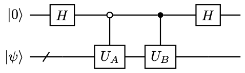
Example 38 (Linear combination of two matrices)
Let \( U_A,U_B\) be two \( n\) -qubit unitaries, and we would like to construct a block encoding of \( T=U_A+U_B\) .
There are two terms in total, so one ancilla qubit is needed. The prepare oracle needs to implement
(440)
so this is the Hadamard gate. The circuit is given by 27, which constructs \( W\in \operatorname{BE}_{\sqrt{2},1}(T)\) .
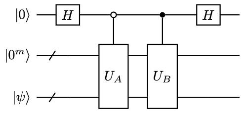
A special case is the linear combination of two block encoded matrices. Given two \( n\) -qubit matrices \( A,B\) , for simplicity let \( U_A\in\operatorname{BE}_{1,m}(A),U_B\in\operatorname{BE}_{1,m}(B)\) . We would like to construct a block encoding of \( T=A+B\) . The circuit is given by 28, which constructs \( W\in \operatorname{BE}_{\sqrt{2},1+m}(T)\) . This is also an example of a linear combination of non-unitary matrices.
Example 39 (Transverse field Ising model)
Consider the following TFIM model with periodic boundary conditions (\( Z_{n}=Z_0\) ), and \( n=2^\mathfrak{n}\) ,
(441)
In order to use LCU, we need \( (\mathfrak{n}+1)\) ancilla qubits. The prepare oracle can be simply constructed from the Hadamard gate
(442)
and the select oracle implements
(443)
The corresponding \( W\in\operatorname{BE}_{\sqrt{2n},\mathfrak{n}+1}(\hat{H})\) .
Example 40 (Block encoding of a matrix polynomial)
Let us use the LCU lemma to construct the block encoding for an arbitrary matrix polynomial for a Hermitian matrix \( A\) in 8.1.
(444)
with \( \left\lVert \alpha\right\rVert _1=\sum_{k\in[K]} |\alpha_k|\) and we set \( K=2^{a}\) . For simplicity assume \( \alpha_k\ge 0\) .
We have constructed \( U_k:=(U_A Z_{\Pi})^k\) as the \( (1,m)\) -block-encoding of \( T_k(A)\) . From each \( U_k\) we can implement the select oracle
(445)
via multi-qubit controls. Also given the availability of the prepare oracle
(446)
we obtain a \( (\left\lVert \alpha\right\rVert _1,m+a)\) -block-encoding of \( f(A)\) .
The need of using \( a\) ancilla qubits, and even more importantly the need to implement the prepare and select oracles is undesirable. We will see later that the quantum signal processing (QSP) and quantum singular value transformation (QSVT) can drastically reduce both sources of difficulties.
Example 41 (Matrix functions given by a matrix Fourier series)
Instead of block encoding, LCU can also utilize a different query model based on Hamiltonian simulation. Let \( A\) be an \( n\) -qubit Hermitian matrix. Consider \( f(x)\in\mathbb{R}\) given by its Fourier expansion (up to a normalization factor)
(447)
and we are interested in computing the matrix function via numerical quadrature
(448)
Here \( \mathcal{K}\) is a uniform grid discretizing the interval \( [-L,L]\) using \( \left\lvert \mathcal{K}\right\rvert =2^{\mathfrak{k}}\) grid points, and the grid spacing is \( \Delta k = 2L/\left\lvert \mathcal{K}\right\rvert \) . The prepare oracle is given by the coefficients \( c_k=\Delta k \hat{f}(k)\) , and the corresponding subnormalization factor is
(449)
The select oracle is
(450)
This can be efficiently implemented using the controlled matrix powers as in 11, where the basic unit is the short time Hamiltonian simulation \( e^{\mathrm{i} \Delta k A}\) . This can be used to block encode a large class of matrix functions.
Theorem 3 (Quantum signal processing, a simplified version)
Consider
(468)
For any \( \widetilde{\Phi} := (\widetilde{\phi}_0, …, \widetilde{\phi}_d) \in \mathbb{R}^{d+1}\) ,
(469)
where \( P\in\mathbb{C}\) satisfy
- \( \deg(P) \leq d\) ,
- \( P\) has parity \( (d \bmod 2)\) ,
- \( |P(x)|\le 1, \forall x \in [-1, 1]\) .
Also define \( -\widetilde{\Phi} := (-\widetilde{\phi}_0, …, -\widetilde{\phi}_d) \in \mathbb{R}^{d+1}\) , then
(470)
Here \( P^*(x)\) is the complex conjugation of \( P(x)\) , and \( U^*_{\widetilde{\Phi}}\) is the complex conjugation (without transpose) of \( U_{\widetilde{\Phi}}\) .
Remark 22
This theorem can be proved inductively. However, this is a special case of the quantum signal processing in 6, so we will omit the proof here. In fact, 6 will also state the converse of the result, which describes precisely the class of matrix polynomials that can be described by such phase factor modulations. In 3, the condition (1) states that the polynomial degree is upper bounded by the number of \( U_A\) ’s, and the condition (3) is simply a consequence of that \( U_{\widetilde{\Phi}}\) is a unitary matrix. The condition (2) is less obvious, but should not come at a surprise, since we have seen the need of treating even and odd polynomials separately in the case of qubitization with a general block encoding. 470 can be proved directly by taking the complex conjugation of \( U_{\widetilde{\Phi}}\) .
Theorem 4 (Quantum eigenvalue transformation with Hermitian block encoding)
Let \( U_A\in\operatorname{HBE}_{1,m}(A)\) . Then for any \( \widetilde{\Phi} := (\widetilde{\phi}_0, …, \widetilde{\phi}_d) \in \mathbb{R}^{d+1}\) ,
(471)
where \( P\in\mathbb{C}\) satisfies the requirements in 3.
Theorem 5 (Quantum eigenvalue transformation with general block encoding)
Let \( U_A\in\operatorname{BE}_{1,m}(A)\) . Then for any \( \widetilde{\Phi} := (\widetilde{\phi}_0, …, \widetilde{\phi}_d) \in \mathbb{R}^{d+1}\) , let
(474)
when \( d\) is even, and
(475)
when \( d\) is odd. Then
(476)
where \( P\in\mathbb{C}\) satisfy the conditions in 3.
Theorem 6 (Quantum signal processing)
There exists a set of phase factors \( \Phi := (\phi_0, …, \phi_d) \in \mathbb{R}^{d+1}\) such that
(481)
if and only if \( P,Q\in\mathbb{C}\) satisfy
- \( \deg(P) \leq d, \deg(Q) \leq d-1\) ,
- \( P\) has parity \( d \bmod 2\) and \( Q\) has parity \( d-1 \bmod 2\) , and
- \( |P(x)|^2 + (1-x^2) |Q(x)|^2 = 1, \forall x \in [-1, 1]\) .
Here \( \deg Q=-1\) means \( Q=0\) .
Remark 23 (\( W\) -convention of QSP)
[8, Theorem 4] is stated slightly differently as
(490)
where
(491)
This will be referred to as the \( W\) -convention. Correspondingly 480 will be referred to as the \( O\) -convention. The two conventions can be easily converted into one another, due to the relation
(492)
Correspondingly the relation between the phase angles using the \( O\) and \( W\) representations are related according to
(493)
On the other hand, note that for any \( \theta\in\mathbb{R}\) , \( U_{\Phi}(x)\) and \( e^{\mathrm{i}\theta Z} U_{\Phi}(x) e^{-\mathrm{i}\theta Z}\) both block encodes \( P(x)\) . Therefore WLOG we may as well take
(494)
In many applications, we are only interested in \( P\in\mathbb{C}\) , and \( Q\in\mathbb{C}\) is not provided a priori. [9, Theorem 4] states that under certain conditions \( P\) , the polynomial \( Q\) can always be constructed. We omit the details here.
Theorem 7 (Quantum signal processing for real polynomials)
Given a real polynomial \( P_{\operatorname{Re}}(x)\in\mathbb{R}\) , and \( \deg P_{\operatorname{Re}}=d>0\) , satisfying
- \( P_{\operatorname{Re}}\) has parity \( d \bmod 2\) ,
- \( |P_{\operatorname{Re}}(x)|\le 1, \forall x \in [-1, 1]\) ,
then there exists polynomials \( P(x),Q(x)\in\mathbb{C}\) with \( \operatorname{Re} P=P_{\operatorname{Re}}\) and a set of phase factors \( \Phi := (\phi_0, …, \phi_d) \in \mathbb{R}^{d+1}\) such that the QSP representation 481 holds.
Corollary 1 (Quantum eigenvalue transformation with real polynomials)
Let \( A\in\mathbb{C}^{N\times N}\) be encoded by its \( (1,m)\) -block-encoding \( U_A\) . Given a polynomial \( P_{\operatorname{Re}}(x)\in\mathbb{R}\) of degree \( d\) satisfying the conditions in 7, we can find a sequence of phase factors \( \Phi\in\mathbb{R}^{d+1}\) , so that the circuit in 32 denoted by \( U_{\Phi}\) implements a \( (1,m+1)\) -block-encoding of \( P_{\operatorname{Re}}(A)\) . \( U_{\Phi}\) uses \( U_A,U_A^{†}\) , m-qubit controlled NOT, and single qubit rotation gates for \( \mathcal{O}(d)\) times.
Remark 24 (Relation between QSP representation and QET circuit)
Although \( O(x)=U_A(x) Z\) , we do not actually need to implement \( Z\) separately in QET. Note that \( \mathrm{i} Z=e^{\mathrm{i} \frac{\pi}{2}Z}\) , i.e., \( Z e^{\mathrm{i} \phi Z}=(-\mathrm{i} ) e^{\mathrm{i} (\frac{\pi}{2}+\phi)Z}\) , we obtain
(495)
where \( \widetilde{\phi}_0=\phi_0,\widetilde{\phi}_j=\phi_j+\pi/2,j=1,…, d\) . For the purpose of block encoding \( P(x)\) , another equivalent, and more symmetric choice is
(496)
When the phase factors are given in the \( W\) -convention, since we can perform a similarity transformation and take \( \Phi=\Phi^W\) , we can directly convert \( \Phi^W\) to \( \widetilde{\Phi}\) according to 496, which is used in the QET circuit in 33.
Example 42 (QSP for Chebyshev polynomial revisited)
In order to block encode the Chebyshev polynomial, we have \( \phi_j=0,j=0,…,d\) . This gives \( \widetilde{\phi}_0=0\) , \( \widetilde{\phi}_j=\pi/2,j=1,…,d\) , and
(497)
According to 496, an equivalent symmetric choice for block encoding \( T_d(x)\) is
(498)
Remark 25 (Other methods for treating QSP with real polynomials)
The proof of [8, Corollary 5] also gives a constructive algorithm for solving the QSP problem for real polynomials. Since \( P_{\operatorname{Re}}=f\in\mathbb{R}\) is given, the idea is to first find complementary polynomials \( P_{\operatorname{Im}},Q\in\mathbb{R}\) , so that the resulting \( P(x)=P_{\operatorname{Re}}(x)+\mathrm{i} P_{\operatorname{Im}}(x)\) and \( Q(x)\) satisfy the requirement in 6. Then the phase factors can be constructed following the recursion relation shown in the proof of 6. We will not describe the details of the procedure here. It is worth noting that the method is not numerically stable. This is made more precise by [10] that these algorithms require \( \mathcal{O}(d\log(d/\epsilon))\) bits of precision, where \( d\) is the degree of \( f(x)\) and \( \epsilon\) is the target accuracy. It is worth mentioning that the extended precision needed in these algorithms is not an artifact of the proof technique. For instance, for \( d\approx 500\) , the number of bits needed to represent each floating point number can be as large as \( 1000\sim 2000\) . In particular, such a task cannot be reliably performed using standard double precision arithmetic operations which only has \( 64\) bits.
Remark 26
When the function \( f(x)\) of interest has singularity on \( [-1,1]\) , the function should first be mollified on a proper subinterval of interest, and then approximated by polynomials. A more streamlined method is to use the Remez exchange algorithm with parity constraint to directly approximate \( f(x)\) on the subinterval. We refer readers to [11, Appendix E] for more details.
Exercise 29
Let \( A,B\) be two \( n\) -qubit matrices. Construct a circuit to block encode \( C=A+B\) with \( U_A\in\operatorname{BE}_{\alpha_A,m}(A),U_B\in\operatorname{BE}_{\alpha_B,m}(B)\) .
Exercise 30
Use LCU to construct a block encoding of the TFIM model with periodic boundary conditions in 195, with \( g\ne 1\) .
Exercise 31
Prove 10.
Exercise 32
Let \( A\) be an \( n\) -qubit Hermitian matrix. Write down the circuit for \( U_{P_{\operatorname{Re}}(A)}\in\operatorname{BE}_{1,m+1}(P_{\operatorname{Re}}(A))\) with a block encoding \( U_A\in\operatorname{BE}_{1,m}(A)\) , where \( P\) is characterized by the phase sequence \( \widetilde{\Phi}\) specified in 3.
Exercise 33
Write down the circuit for LCU of Hamiltonian simulation.
Exercise 34
Using QET to prepare the Gibbs state.
Definition 4 (Generalized matrix function {[12, Definition 4]})
Given \( A\in\mathbb{C}^{N\times N}\) with singular value decomposition 513, and let \( f: \mathbb{R} \rightarrow \mathbb{\mathbb{C}}\) be a scalar function such that \( f\left(\sigma_{i}\right)\) is defined for all \( i\in[N]\) . The generalized matrix function is defined as
(515)
where
Definition 5
Under the conditions in 4, the left and right generalized matrix function are defined respectively as
(516)
Proposition 12
The following relations hold:
(517)
and
(518)
Remark 27
By approximating any continuous function \( f\) using polynomials, and using the LCU lemma, we can approximately evaluate \( f^{\diamond}(A)\) for any odd function \( f\) , and \( f^{\triangleright}(A)\) for any even function \( f\) . This may seem somewhat restrictive. However, note that all singular values are non-negative. Hence when performing the polynomial approximation, if we are interested in \( f^{\diamond}(A)\) , we can always use first perform a polynomial approximation of an odd extension of \( f\) , i.e.,
(535)
and then evaluate \( g^{\diamond}(A)\) . Similarly, if we are interested in \( f^{\triangleright}(A)\) for a general \( f\) , we can perform polynomial approximation to its even extension
(536)
and evaluate \( g^{\triangleright}(A)\) .
Theorem 8 (Quantum singular value transformation with real polynomials)
Let \( A\in\mathbb{C}^{N\times N}\) be encoded by its \( (1,m)\) -block-encoding \( U_A\) . Given a polynomial \( P_{\operatorname{Re}}(x)\in\mathbb{R}\) of degree \( d\) satisfying the conditions in 7, we can find a sequence of phase factors \( \Phi\in\mathbb{R}^{d+1}\) , so that the circuit in 37 denoted by \( U_{\Phi}\) implements a \( (1,m+1)\) -block-encoding of \( P^{\diamond}_{\operatorname{Re}}(A)\) if \( d\) is odd, and of \( P^{\triangleright}_{\operatorname{Re}}(A)\) if \( d\) is even. \( U_{\Phi}\) uses \( U_A,U_A^{†}\) , m-qubit controlled NOT, and single qubit rotation gates for \( \mathcal{O}(d)\) times.
Theorem 9 (Quantum singular value transformation with real polynomials and projectors)
Let \( \widetilde{U}_A\) be a \( (n+m)\) -qubit unitary, and \( \Pi,\Pi'\) be two \( (n+m)\) -qubit projectors of rank \( 2^n\) . Define the basis \( \mathcal{B},\mathcal{B'}\) according to Label eqn:qsvt_proj_basis_b,eqn:qsvt_proj_basis_bp not found., and let \( A\in\mathbb{C}^{N\times N}\) be defined in terms of the matrix representation in 565. Given a polynomial \( P_{\operatorname{Re}}(x)\in\mathbb{R}\) of degree \( d\) satisfying the conditions in 7, we can find a sequence of phase factors \( \Phi\in\mathbb{R}^{d+1}\) to define a unitary \( U_{\Phi}\) satisfying
(571)
if \( d\) is odd, and
(572)
if \( d\) is even. Here \( \Pi'\ket{\perp_j'}=0\) , \( \Pi\ket{\perp_j}=0\) , and \( U_{\Phi}\) uses \( \widetilde{U}_A,\widetilde{U}_A^{†}\) , \( \operatorname{C} _{\Pi} \operatorname{NOT} , \operatorname{C} _{\Pi'} \operatorname{NOT} \) , and single qubit rotation gates for \( \mathcal{O}(d)\) times.
Proposition 13 (Fixed-point amplitude amplification)
Let \( \widetilde{U}_A\) be an \( n\) -qubit unitary and \( \Pi'\) be an \( n\) -qubit orthogonal projector such that
(582)
Then there is a \( (n+1)\) -qubit unitary circuit \( U_{\Phi}\) such that
(583)
here \( U_{\Phi}\) uses the gates \( \widetilde{U}_A,\widetilde{U}_A^{†}, \operatorname{C} _{\Pi'} \operatorname{NOT} , \operatorname{C} _{\ket{\varphi_0}\bra{\varphi_0}} \operatorname{NOT} \) and single qubit rotation gates for \( \mathcal{O}(\log(1/\epsilon) \delta^{-1})\) times.
Exercise 35 (Robust oblivious amplitude amplification)
Consider a quantum circuit consisting of two registers denoted by \( a\) and \( s\) . Suppose we have a block encoding \( V\) of \( A\) : \( A=(\bra{0}_a\otimes I_s)V(\ket{0}_a\otimes I_s)\) . Let \( W=-V(\mathrm{REF}\otimes I_s)V^{\dagger}(\mathrm{REF}\otimes I_s)V\) , where \( \mathrm{REF}=I_a-2\ket{0}_a\bra{0}_a\) . (1) Within the framework of QSVT, what is the polynomial associated with the singular value transformation implemented by \( W\) ? (2) Suppose \( A=U/2\) for some unitary \( U\) . What is \( (\bra{0}_a\otimes I_s)W(\ket{0}_a\otimes I_s)\) ? (3) Explain the construction of \( W\) in terms of a singular value transformation \( f^{\diamond}(A)\) with \( f(x)=3x-4x^3\) . Draw the picture of \( f(x)\) and mark its values at \( x=0,\frac12,1\) .
Exercise 36 (Logarithm of unitaries)
Given access to a unitary \( U=e^{\mathrm{i} H}\) where \( \left\lVert H\right\rVert \le \pi/2\) . Use QSVT to design a quantum algorithm to approximately implement a block encoding of \( H\) , using controlled \( U\) and its inverses, as well as elementary quantum gates.
References
[1] Quantum computation and quantum information 2000
[2] Fast amplification of QMA Quantum Inf. Comput. 2009 9 11 1053–1068
[3] Optimal quantum eigenstate filtering with application to solving quantum linear systems Quantum 2020 4 361
[4] Quantum algorithm for linear systems of equations Phys. Rev. Lett. 2009 103 150502
[5] Matrix computations Johns Hopkins Univ. Press 2013 Baltimore Fourth
[6] Random circuit block-encoded matrix and a proposal of quantum LINPACK benchmark Phys. Rev. A 2021 103 6 062412
[7] Lecture Notes on Quantum Algorithms 2021
[8] Quantum singular value transformation and beyond: exponential improvements for quantum matrix arithmetics Proceedings of the 51st Annual ACM SIGACT Symposium on Theory of Computing 2019 193–204
[9] Quantum singular value transformation and beyond: exponential improvements for quantum matrix arithmetics arXiv:1806.01838 2018
[10] Product decomposition of periodic functions in quantum signal processing Quantum 2019 3 190
[11] Efficient phase factor evaluation in quantum signal processing Phys. Rev. A 2021 103 042419
[12] Computation of Generalized Matrix Functions SIAM J. Matrix Anal. Appl. 2016 37 836–860